Money And Statistical Delusions
Authored by Alasdair Macleod via GoldMoney.com,
“I can prove anything with statistics, except the truth”
— Lord Canning, c. 1819
Does Canning’s aphorism still hold true, given that data collection and statistical analysis have progressed beyond all recognition in the last two hundred years? This article tests that proposition.
It is still true, because of the interests for which statistics are deployed. We know, or should know, that CPI indexation of prices fails to reflect the true rate of decline in the purchasing power of fiat currencies. That is at least a simple case of governments saving money on indexation. But being economical with the statistical truth is a far wider practice encompassing input suppression, misleading deployment, and their use to support beliefs and preferred outcomes instead of backing up properly reasoned economic and monetary a priori theory.
This article finds that the application of all these methods corrupt monetary statistics, including the three principal components of the equation of exchange. This analysis is sparked by recent changes to the definition of M1 money supply in the US.
Introduction
Monetarists have long held that there is a relationship between changes in the quantity of circulating currency and the general level of prices. It is not the only factor governing the relation, but it has been generally established to be true. So persuasive is the theoretical case, that no one — not even modern monetary theorists — deny it. We generally assume that the monetary statistics, the sheet anchor to the equation of exchange that emerged over a century ago, are reliable. But even monetary statistics whose components drop out of accounting identities end up being sliced and diced at the behest of the authorities, raising the question as to what we should regard as money at a time of unprecedented peacetime global monetary expansion. And the monetary policy planners moving the goal posts question by their actions the macroeconomic habit of relying solely on statistical evidence for predicting outcomes.
In February, the Fed changed the definition of M1 to include “Savings deposits” and “Other checkable deposits”. They are now combined and reported as “Other liquid deposits”. The effect is to increase M1 but to leave M2 unchanged, as illustrated in Figure 1.

The change accepts the reality, long recognised in the Austrian school’s definition of money supply (AMS), that depositors and banks assume savings accounts are just another form of money available for spending on day-to-day transactions. Monetary policy planners generally circumvent such considerations, looking at monetary definitions from their policy viewpoint instead of the perspective of money’s users.
For statistics junkies, there is a disadvantage in that the new M1 is only readily available as a retrospective monthly average instead of a more current weekly average. This has the effect of under recording the increase of M1 in this statistic at times of rapidly rising monetary inflation. And importantly, M1 is so much modified by these changes as to be rendered useless as a statistical record of monetary inflation.
This raises other questions, such as should we regard broad money or narrow money as the primary indicator of changes in the money supply? And, more deeply, should we ignore the statistical detail and try to understand money from an a priori analysis of the theory of exchange? This is the key difference in the approach of establishment monetarists compared with the Austrian school. Monetarists today, in common with other macroeconomic schools, test propositions by statistical correlation, thereby avoiding the necessity of sound theoretical analysis. Consequently, the definition of money rarely progresses beyond simplistic propositions. And its true use value, which is defined by less predictable human action, is ignored.
The Austrian school generally disregarded the statistical approach to money, until Murray Rothbard attempted to define circulating currency solely in the context of US monetary statistics, work that was consolidated by Joseph Salerno.[i] But slotting different monetary statistics into any combination has never been standardised, so what applies in America, which cannot be precisely defined anyway, doesn’t apply elsewhere. Nor does it when the makeup of a monetary component is altered, excluded or included, such as the current modifications to M1.
Therefore, whatever statistical evidence there is can only be used to corroborate a theoretical analysis, and not be accepted as prima facie evidence. As Lord Canning put it two centuries ago, you can prove anything with statistics but the truth.
Defining money
A theoretical approach to understanding money must start by defining it. This definition is taken from the glossary to von Mises’s Human Action:“The most commonly used medium of exchange in society. A community’s most marketable economic good, which people seek primarily for the purpose of later exchanging units of it for the goods or services they prefer. The circulating media most readily accepted for the payment for goods, services and outstanding debts. Money is an indispensable factor in the development of the division of labour and the resulting indirect exchanges upon which modern civilisation is based.”In other words, money is the medium that links production with consumption through the division of labour. It must be immediately available for that purpose. That certainly includes cash in circulation and money in the bank. Correctly, it is now argued by the Fed that because in practice savings are instantly available to bank depositors, that they are cash equivalents. But there are other important aspects of money, such as unspent government balances. Because that can be drawn down at any time, it is money as well, just as if it were money due to an ordinary depositor. But that is not included in the Fed’s definition of M1 (renamed M1 SL), which is an important omission given recent balances on the government’s general account of as much as $1.7 trillion. If, as well as savings deposits, unspent government balances had been included, M1 SL money supply would have looked more like Rothbard’s Austrian money supply (AMS) in Figure 2.
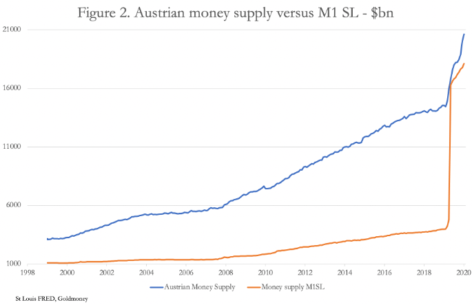
There are good theoretical grounds behind the Austrian money supply calculation, but the absence of the government’s general account in the official M1 calculation disqualifies it from being a true reflection of cash and cash alternatives available for spending. Consequently, official M1 has not yet caught up with AMS, having risen from $3,977bn in January 2020 to $18,105 exactly a year later, an increase of 355%. Over the same timescale AMS rose from $14,082 to $20,614, an increase of 46% — less dramatic perhaps, but genuine.
When it comes to managing expectations, a genuine increase in narrow money of 46% is of greater concern than a far larger increase due to changes in the statistic. This appears to be the reason for the Fed’s part-conversion to Austrian money supply. But they chose a halfway house, which signals perhaps less of a comprehension about what money represents to the wider public and more of a desire to conceal the true state of monetary affairs. And by suppressing interest rates, monetary policy attempts to increase the circulation of money which, the planners appear to believe, would otherwise sit in bank deposits unutilised. The fact that bank deposits are the backing for bank credit whose expansion is also desired escapes this line of reasoning, but that does not stop planners trying to increase the circulation of money.
The velocity myth
Even with M1 money supply at a lower figure that AMS, velocity of circulation is close to unity. Velocity is a widely accepted concept, used as a statistic to promote macroeconomic discourse. The St Louis Fed defines it as follows:
The velocity of money is the frequency at which one unit of currency is used to purchase domestically produced goods and services within a given time period. In other words, it is the number of times one dollar is spent to buy goods and services per unit of time. If the velocity of money is increasing, then more transactions are occurring between individuals in an economy.
This is patently untrue. For it to be correct there would be no relation between production and consumption, and consumers would somehow end up with money to spend without earning it. Money-printing might appear to satisfy this condition, because some money is produced out of thin air instead of being genuinely earned by economic actors. It does not excuse this calumny. What makes this statistical approach acceptable to neo-Keynesians is the denial of Say’s law, which describes the rationale behind the division of labour and points out that money is the most marketable intermediate good whose primary function permits production to be turned into consumption.
If there is one concept that illustrates the difference between a top-down macro-economic approach and the reality of everyday life it is concepts such as the velocity of circulation of money.
Compare the following statements:
“Whenever the interest rate on financial assets is low, the desire to hold money falls as people try to exchange it for other goods or financial assets. As a result, the velocity of circulation rises. Hence, when the money demand is low, the velocity will be high. Conversely, when the opportunity cost/alternate cost is low, money demand is high, and the velocity of circulation is low”.
– Corporate Finance Institute – What is velocity of circulation?
This is in line with monetary planners’ policy of interest rate suppression. They suppress the interest rate to encourage monetary circulation. But if this is valid, then the opposite cannot be true. Yet today, falling velocity to approximately unity with GDP has been accompanied by falling interest rates, even to the zero bound, disproving macroeconomic assumptions.
The next statement is from an economist in the classical, Austrian tradition:
“The mathematical economists refuse to start from the various individuals’ demand for and supply of money. They introduce instead the spurious notion of velocity of circulation according to the pattern of mechanics.”
– Ludwig von Mises, Human Action.
In effect, von Mises is saying it is free markets that decide how money is used, not state management of interest rates.
The mathematical economist might attempt to argue that interest rates affect the relationship between consumption and savings, with higher rates reducing immediate consumption. But that is a red herring, because GDP includes business investment and government spending financed by savings and therefore money not spent on direct consumption. To further understand the errors in the velocity concept we must delve into its origins.
The notion of velocity of circulation arose from the quantity theory of money, which links changes in the quantity of money to changes in the general level of prices. This is set out in the equation of exchange. The basic elements are money, velocity and total spending, represented by GDP. The following is the simplest of a number of ways it has been expressed:
Money x Velocity = Total Spending (or GDP)
Assuming we can measure both the quantity of money and total spending, we end up with velocity. But this does not tell us why velocity might vary: all we know is that it must vary in order to balance the equation. You could equally state that two completely unrelated metrics can be put into a mathematical equation, so long as a variable is included whose only function is to always make the equation balance. In other words, velocity is not a valid expression of the relationship between money and prices; it is merely there to balance an equation that otherwise does not exist.
Von Mises’s criticism is based on the philosopher’s logic that economics is a social and not a physical science. Therefore, mathematical relationships must be strictly confined to accounting and not be confused with resolving economic issues. Unfortunately, economists and commentators have the concept of velocity so ingrained in their thinking that this vital point escapes them.
The only apparent certainty in the equation of exchange is the quantity of money, assuming it is all recorded. No one seems to allow for unrecorded money or assets that can be assumed to be held as readily accessible cash alternatives. Furthermore, if the money is sound, as it was when the quantity theory of money was devised, one could deduce that after a time lag to allow it to fully circulate, an increase in its quantity would more directly tend to raise prices, because changes in the general level of personal liquidity in a population whose money is sound tend to be more stable than that under a fiat money regime.
Today we no longer have sound money, whose purchasing power was regulated by human preferences across national boundaries without impediment. Instead, we have fiat currencies whose purchasing power is formalised in foreign exchanges and corrupted by state intervention. An illustrative example of the consequences is given to us from the Icelandic krona, which on 8th October 2008 suddenly halved in value, which had nothing to do with changes in the quantity of money, its velocity of circulation or Iceland’s GDP.
In economic history, Iceland’s currency collapse was not an isolated event. The purchasing power of a fiat currency varies continually, even to the point of losing it altogether irrespective of changes in its quantity. The truth of the matter is that the utility of a fiat currency in the short-term is entirely dependent on the subjective opinions of individuals expressed through markets and has little to do with a mechanical quantity relationship. In this respect, merely the potential for unlimited currency issuance or a change in perceptions of the issuer’s financial stability, as Iceland discovered, can be enough to destabilise it.
According to the equation of exchange, this is not how things should work. The order of events is first you have an increase in the quantity of money and then prices rise, because monetarist logic states that prices rise as a result of the extra money being spent, not as a result of money yet to be spent. With a mechanical theory there can be no room for subjectivity.
It is therefore nonsense to conclude that velocity is a vital signal of some sort. Linking the relationship between changes in the quantity of money to the effect on prices is certainly more justified in the case of sound money, backed by and freely exchangeable into gold coin. But no material changes to the original concept have allowed for the different characteristics between sound and fiat moneys.
Monetarist theory in its current form is at the very least still a red herring until monetarists finally discover velocity is no more than a factor to make their equation balance. It is indicative of the false mechanisation of human behaviour by modern macro-economists. However, it should also be noted that it is impossible to square the concept of velocity of circulation with one simple fact of everyday life: we earn our salaries and make our profits once and we dispose of them. That’s a constant velocity of exactly one, assuming no change in cash levels over the period under consideration.
This is the irrefutable conclusion of Say’s law. But it was dismissed by Keynes in his General Theory to make way for his macroeconomic fallacies.
The implications of monetary expansion
Following Rothbard’s logic, that money and its immediately encashable equivalents in the mind’s eye of the individual are together the true money supply, we can see from Figure 2 above that in an economy whose annualised GDP is estimated at $21.5 trillion and with Austrian money supply standing at $20.6 trillion, it is 95% of all transactions, suggesting that the average economic actor holds almost a year’s worth of cash liquidity. Clearly, as a result of continual monetary expansion, the US economy is awash with money that hardly, on average, circulates.
In addition to AMS, there is credit money, which is rightly excluded, because being on the other side of a bank’s balance sheet from deposits it is not necessarily available for immediate payments — the bank can always restrict issues of undrawn credit. In this category we can also include shadow banking balances. And payments by credit card are not instantaneous, the payment for goods being deferred by up to a month, so these and similar credit facilities must be excluded as well.
Obviously, there is a link between bank credit expansion and the growth of deposits, raising the question of whether deposits so created should be included in AMS. The answer is no distinction should be made between deposits and those that result from credit expansion, because for the user all bank deposits are regarded as money, whatever their origin.
Left to free markets and sound money, money would undoubtedly be scarce, but plentiful enough to act as the medium of exchange between production and consumption. Therefore, fiat dollar money existing in the quantity that it does is the consequence of easy money policies. Rather than assuming that negative rates will stimulate the population to use it, which is undoubtedly behind official thinking, efforts should be put into considering how to reduce the danger of excess money being unexpectedly mobilised for goods.
The inconvenience of the current position is explained by von Mises’s description of money’s role as “a community’s most marketable economic good, which people seek primarily for the purpose of later exchanging units of it for the goods or services they prefer”. The risk is that substantial quantities of money will be mobilised for that function if people decide to reduce their relationship between owning money in reserve and owning goods which they do not immediately need.
But with covid lockdowns knocking out swathes of industrial production, the goods and services are not available to satisfy this potential demand. Consequently, prices can only rise significantly until the money relationship rebalances. In other words, nominal GDP, being no more than a money total, which we discuss below, will appear to rise dramatically. And with official estimates of price inflation blatantly suppressed, officially recorded “real” GDP will be declared as evidence of the success of monetary policy in rescuing the economy. But remember Canning’s aphorism: I can prove anything with statistics, except the truth…
GDP fallacies
So far, we have shown the errors in official monetary statistics and explained why velocity of circulation is meaningless. Ignorance over velocity of circulation can perhaps be understood because the reasoning behind the equation of exchange predates macroeconomics and is a belief only partially backed by reasoning. We now turn our attention to the third and final component of the equation of exchange. Ignorance cannot so easily be justified about GDP, which was invented in the 1930s, and whose only practical use is to indicate to the state the potential for tax revenues. Its role in the equation of exchange as a substitute for prices is misleading.
GDP is no more than a money total of recorded transactions during a period, usually over a year or annualised. It does not reveal the quality of transactions and economic progress as commonly supposed. It is consistent with what von Mises described as an evenly rotating economy. Again, we can refer to the glossary in his Human Action:
“An imaginary economy in which all transactions and physical conditions are repeated without change in each similar cycle of time. Everything is imagined to continue exactly as before, including all human ideas and goals. Under such fictitious constant repetitive conditions, there can be no net change in any supply or demand and therefore there cannot be any change in prices.”
By deflating it for officially recorded price inflation, GDP appears to meet all the conditions of an evenly rotating economy. Plainly, it does not accord with reality. Furthermore, if the quantity of money was constant and the balance of trade meant it was contained within a community, then that community’s GDP would also remain constant. The logic of this statement is unchallengeable.
Therefore, numerical increases in an evenly rotating economy must come from the money side. In other words, if the quantity of money and credit in an economy is increased, so will GDP. And none of its increase can be attributed to an improvement in economic conditions, because it is modelled on a constantly rotating economy. This is clearly illustrated by removing monetary expansion from the GDP statistic, as illustrated in Figure 3.

Deflating nominal GDP by broad money tells us that US GDP is indeed evenly rotating and has been doing so with not much variation for over four decades. The only notable exceptions were following the Lehman crisis when the US economy entered a brief downturn greater than the expansion of broad money, and in 2020. The latter reflects a large increase in unemployed and underemployed individuals who are still receiving direct payments from the government while locked down due to the coronavirus.
The severity of economic contraction last year was thereby concealed by the expansion of broad money. And its further expansion since the last data point (Q3 2020) will continue to mask the true depth of the economic slump. And for further confirmation, Figure 4 shows the same relationship between GDP and money supply for the UK, where similar factors are at play.

Establishment economists make no differentiation between the real economy and GDP. One never hears or reads any distinction between the two, and Mises’s evenly rotating economy is almost exclusively confined to a few unread pre-Keynesian texts. But its expansion being linked entirely to increases in the money supply reveals that its increase is completely meaningless. But then, monetary and economic policies need to deliver something to justify their existence, not to mention the livings of all the government economists and statisticians and of their opposite numbers in financial and banking institutions.
But with all the inflation money being funnelled into economies today, there can be little doubt that GDP will increase accordingly. But as the charts in Figures 3 and 4 show, with productive capacity cut, the US and UK economies are in a depression.
Canning calls out to us. Forget the statistics, just look around you.
Tyler Durden
Sun, 03/07/2021 – 22:00
from ZeroHedge News https://ift.tt/2Orfq3f